Differential Gene Expression Analysis

Differential Gene Expression Analysis

Multiple tools across multiple programming languages can be used to perform Differential Gene Expression (DGE) analysis. When using R and the Bioconductor packages, the main three are limma, edgeR and DESeq2.

In this guide we will be looking at the limma package. The advantage of using limma over the other tools is its higher flexibility, specially when it comes to more complex experimental designs. Since here we will only be looking at a trivial control vs. condition comparison any of the tools can easily be used, it will still be interesting to see how to use limma in this scenario.

limma stands for linear models and differential expression for microarray data, and as the name entails it was first designed for the analysis of microarray expression data. It has been updated since to also take into allow for the analysis of RNA-Seq data. limma was created by the same team behind edgeR, therefore some of the functions are common to both tools and it is sometimes required to also import edgeR into the limma pipeline.

Two main resources were used to inspire this pipeline, the main documentation for the limma package user’s guide and the RNA-seq analysis is easy as 1-2-3 with limma, Glimma and edgeR paper by Law et al.¹

1. Preparing Input Data

Before starting DGE analysis it is necessary to create a DGEList object, i.e., the data format used by the edgeR and limma software to organize and perform DE analysis. The advantage of using this object is that it easily allows to filter data across all 3 data objects described below. So for example if I remove all genes that are annotated as being from the mitochondrial chromosome in the rowData file, this will also remove them from the assays dataframe. The same goes for example if I want to remove all samples labeled as males from the colData object, doing so, as we’ll see in the code below, will also remove them from the assays data frame.

The following figure explains some of the components of the SummarizedExperiment object, a similar, often precursor object to DGEList. In fact, the same people that developed edgeR also created a function to convert one object into the other, SE2DGEList. The only data the DGEList object requires to be created is the assays data frame, which contains the gene count data output by STAR and HTSeq. You can refer to the gen_star_results.py python script file, for an example of how to transform the STAR outputs into the assays data frame. In the scope of this tutorial we will also be integrating the colData and rowData objects to it, which respectively contain the samples and the features (genes) metadata.

Figure 1: The integrative data container SummarizedExperiment()
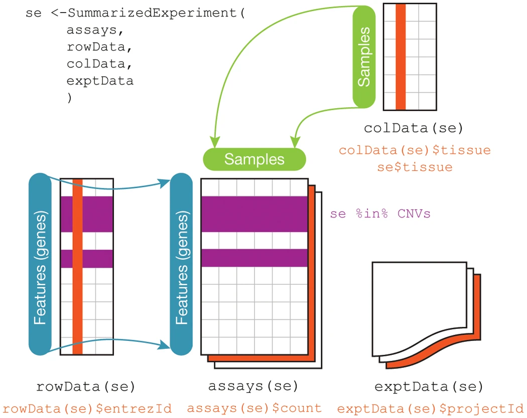
Figure 2 from the Huber et al., 2015 Nature methods paper.

The assays data contains the actual gene expression data organized by features (genes) in rows and the samples as columns, see the star_results.csv file. The colData file should contain the sample names or identification as rows IN THE SAME ORDER as the column names in the assays data and metadata as columns, see the conditions_df.csv file. The rowData contains extra information about the genes (features), such as chromosome number, other types of gene names (ensembl, entrez gene id, etc.), protein name, etc. IN THE SAME ORDER as the row names in the assays data frame. For this analysis this data was acquired from the ensembl’s online biomart tool. This tools let’s the user select and download specific features metadata from an organism’s database. Here we used the Mouse GRCm38 database, see the mm10_biomart_annotated_genes.csv file. It can also be used programmatically as a Bioconductor package.

The choice of metadata to include will vary with each experiment, this data can be used to cluster, label and better understand the expression data and is therefore very important.

2. Performing the DE analysis in R:

Below we will go through the steps of a typical Control (Ctrl) vs. Condition (Cond) bulk RNA-Seq differential gene expression analysis. You can find the Rscript file with only the code content here.

2.1 Data import and setup:

Loading the required packages:

library(limma)
library(Glimma)
library(edgeR)
library(RColorBrewer)
library(kableExtra)

Setting the working directory to the folder containing the analysis files. Refer to __ for a sample/suggested directory tree.
setwd("C:/Users/path_to_analysis_directory/rna-seq_workflow/scripts/dge_analysis")

Then import the required files:

• Experimental variables dataframe (colData):
  colData_df = read.csv('../../data_files/limma_voom/conditions_df.csv')

• STAR gene count output results dataframe (assays):
  assays_df = read.csv('../../data_files/limma_voom/star_results.csv', row.names=1)

• Biomart gene annotation file (rowData):
  rowData_df = read.csv("../../data_files/limma_voom/mm10_biomart_annotated_genes.csv")

2.2 Creating the DGEList Object:

N.B.: The remove.zeros=TRUE parameter for the DGEList removes all genes for which the expression is zero in all samples. From a biological point of view, genes that are not expressed at a biologically meaningful level in any condition are not of interest and are therefore best ignored. From a statistical point of view, removing low count genes allows the mean-variance relationship in the data to be estimated with greater reliability and also reduces the number of statistical tests that need to be carried out in downstream analyses looking at differential expression.¹ There were 13902 genes with 0 count in total and it represented 25% of the gene set.

# dataframe with factors:
colData_df <- data.frame(sample_id = colData_df$sample_id, 
                         subject = substr(colData_df$sample_id, 1, 5), 
                         treat = colData_df$treatment, 
                         sex = colData_df$sex, 
                         roi = colData_df$region
)


# Group
group = factor(colData_df$treat)

# remove.zeros=TRUE gets rid of genes with 0 counts
dge <- DGEList(counts=assays_df, group=group, remove.zeros=TRUE)

# add factors to DGEList object
dge$samples$subject <- factor(colData_df$subject)
dge$samples$treat <- factor(colData_df$treat)
dge$samples$sex <- factor(colData_df$sex)
dge$samples$roi <- factor(colData_df$roi)


# add annotations, same order as in DGE object gene ids:
annotations_df <- annotations_df[match(rownames(dge), annotations_df$ensembl_gene_id), ]
dge$genes <- annotations_df

2.3 Filtering and Design Matrix

It’s in this section that we filter the DGEList object as described above, i.e. using the metadata values in colData and/or rowData. Here we decided to only keep the genes annotated as being protein coding for the gene_biotype annotation from the ensembl database (rowData). They amount to 19511 and therefore account for roughly 35% of the original gene set.

# Keep protein coding genes only:
keep <- dge$genes$gene_biotype == 'protein_coding'
dge <- dge[keep, ]

If we were to filter using the samples metadata (colData), for instance to only keep Females, the commands would be similar:

# Only keep female samples:
dge <- dge[, which(dge$samples$sex=="F")]

Creating the Design Matrix, the reason we create the design matrix now is that it is required as a parameter by the filterByExpr() function. The latter provides an automatic way to filter genes while keeping as many genes as possible with counts considered worthwhile.¹ The package suggests keeping between 10 and 15 read counts as a minimum number of samples, where the number of samples is chosen according to the minimum group sample size. The actual filtering uses CPM (Counts per million) values rather than counts in order to avoid giving preference to samples with large library sizes. For our dataset, the median library size is about 29 million reads and we chose to keep 10 as a min.count value, since our analysis has enough replicates (6) to account for potential outliers. Since 10/29 = 0.344, the function keeps genes that have a CPM of 0.344 or more in at least 6 samples. A biologically interesting gene should be expressed in at least six samples because all the cell type groups have six replicates. The cutoffs used depend on the sequencing depth and on the experimental design. If the library sizes had been larger, then a lower CPM cutoff would have been chosen, because larger library sizes provide better resolution to explore more genes at lower expression levels. Alternatively, smaller library sizes decrease our ability to explore marginal genes and hence would have led to a higher CPM cutoff. Using this criterion, the number of genes is reduced to 15025 of the original 55421 genes.

design = model.matrix(~ 0 + group + roi + sex, data = dge$samples)
# Remove "group" from design column names:
colnames(design) = sub("group", "", colnames(design))

# Remove Lowly Expressed Genes:
keep <- filterByExpr(dge, design=design, min.count=10)
dge <- dge[keep,, keep.lib.sizes=FALSE]

About design matrices: The modelling process requires the use of a design matrix (or model matrix) that has two roles: 1) it defines the form of the model, or structure of the relationship between genes and explanatory variables, and 2) it is used to store values of the explanatory variable(s)(Smyth 2004, 2005; Glonek and Solomon 2004). Although design matrices are fundamental concepts that are covered in many undergraduate mathematics and statistics courses, their specific and multi-disciplinary application to the analysis of genomic data types through the use of the R programming language adds several layers of complexity, both theoretically and in practice. For more information on the appropriate design matrix set up for differential expression analyses specific to using the limma, refer to this online guide by Law et al. (2020) from which the paragraph above is an excerpt.

2.4 Background Gene List Generation (Optional)

At this point in the analysis, one can decide to generate a background gene list for later use with pathway analysis tools (see the Pathway Enrichment Analysis page for more information). The goal of a background list is to not use the entire “universe” i.e., all genes in the organism, to check for significant enrichment whilst performing pathway enrichment analysis. Instead, only using the genes that are relevant in the data for the comparison we’re making. For the M vs. F comparison in the ACC for instance, the only genes relevant are the ones that passed the filtering thresholds (first removing all genes with 0 expression, i.e., keeping only the genes expressed in that particular brain region, then only keeping the protein coding genes and those having passed a minimum expression value, calculated with the filterByExpr() function). The aim being to allow a more precise evaluation of functional enrichment.

# Save background genes list to file:
write.csv(dge$genes, "../../data_files/limma_voom/bg_list.csv", row.names=FALSE)

2.5 Normalization

CPM normalization, which is applied above normalizes the counts, or the number of reads that align to a particular feature after correcting, for sequencing depth and transcriptome composition bias. There is however another most important technical influence on differential expression that is less obvious. Indeed, RNA-Seq provides a measure of the relative abundance of each gene in each RNA sample, but does not provide any measure of the total RNA output on a per-cell basis. This commonly becomes important when a small number of genes are very highly expressed in one sample, but not in another. The highly expressed genes can consume a substantial proportion of the total library size, causing the remaining genes to be under-sampled in that sample. Unless this RNA composition effect is adjusted for, the remaining genes may falsely appear to be down-regulated in that sample.² The calcNormFactors() function normalizes for RNA composition by finding a set of scaling factors for the library sizes that minimize the log-fold changes between the samples for most genes. The default method for computing these scale factors uses a trimmed mean of M-values (TMM) between each pair of samples.³ We call the product of the original library size and the scaling factor the effective library size. The effective library size replaces the original library size in all downstream analyses. TMM is recommended for most RNA-Seq data where the majority (more than half) of the genes are believed not differentially expressed between any pair of the samples, see the edgeR: differential analysis of sequence read count data user’s guide for more information.³ This bioconductor forum post can also be informative.

The log-CPM distributions are similar throughout all samples within this dataset. The normalization factors of all the libraries multiply to unity. A normalization factor below one indicates that a small number of high count genes are monopolizing the sequencing, causing the counts for other genes to be lower than would be usual given the library size. As a result, the effective library size will be scaled down for that sample. For this dataset the effect of TMM-normalization is mild, as evident in the magnitude of the scaling factors, which are all relatively close to 1, see on the figure below:

# Compute composition normalization factors to scale the raw library sizes with TMM method:
dge <- calcNormFactors(dge, method = "TMM")

Figure 2: Distribution of Per Sample Normalization Factors

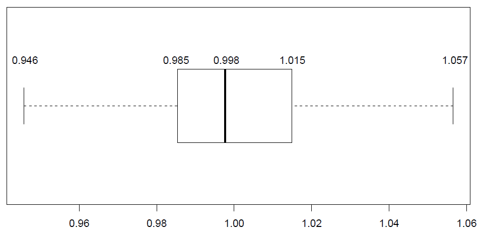
It is important to note that TMM does not change gene expression counts or library sizes, it merely creates a new column: (samples$norm.factors) of scaling factors to be automatically used downstream in the analysis when applying edgeR or limma functions. For example, edgeR’s cpm() function (this is what is referred to in the edgeR package as model normalization). We can see the effect of the TMM normalization by plotting the log-cpm distributions before and after normalization as in the figure below. The distributions are slightly different pre-normalization and are similar post-normalization.

2.6 Unsupervised Clustering with MDS plots

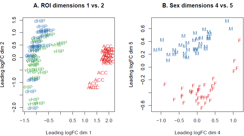
Similarly to the Principal component analysis (PCA), the multi-dimensional scaling (MDS) plot shows similarities and dissimilarities between samples in an unsupervised manner so that one can visualize how differential expression is behaving in-between different samples before carrying out more formal testing. This is both an analysis and a quality control step to explore the overall differences between the expression profiles of the different samples. Distances on an MDS plot of a DGEList object correspond to leading log-fold-change between each pair of samples. Leading log-fold-change is the root-mean-square average of the largest log2-fold-changes between each pair of samples. The MDS plot is also useful to identify potential sample outliers. The first dimension represents the leading-fold change that best separates samples and explains the largest proportion of variation in the data, with subsequent dimensions having a smaller effect and being orthogonal to the ones before it. Since our experimental design involves multiple factors, we examined each factor over several dimensions. If samples cluster by a given factor in any of these dimensions, it suggests that the factor contributes to expression differences and is worth including in the linear modelling. On the other hand, factors that show little or no effect may be left out of downstream analysis. In this dataset, samples can be seen to cluster well within brain region groups over dimension 1 and 2, and then separate by sex over dimension 5.

par(mfrow=c(1,2))

# ROI (Brain Regions) on dimensions 1 vs. 2:
col.group <- dge$samples$roi # gen color group vector
levels(col.group) <-  brewer.pal(nlevels(col.group), "Set1") # assign colors as factors
col.group <- as.character(col.group)
mds <- plotMDS(dge, labels=dge$samples$roi, col=col.group, dim.plot=c(1,2), main="A. ROI dimensions 1 vs. 2")

# Sex on dimensions 4 vs. 5:
col.group <- dge$samples$sex # gen color group vector
levels(col.group) <-  brewer.pal(nlevels(col.group), "Set1") # assign colors as factors
col.group <- as.character(col.group)
mds <- plotMDS(dge, labels=dge$samples$sex, col=col.group, dim.plot=c(4,5), main="B. Sex dimensions 4 vs. 5")

Figure 3: MDS Plots of log-CPM Values

Exquisitely, the Glimma package offers the convenience of an interactive MDS plot where multiple dimensions can be explored. It generates an HTML page with an MDS plot in the left panel and a scree plot showing the proportion of variation explained by each dimension in the right panel. Clicking on the bars of the scree plot changes the pair of dimensions plotted in the MDS plot, and hovering over the individual points reveals the sample label. The colour scheme can be changed as well to highlight the different factors to look at, for example in this case: brain regions (roi), sex or treatment vs. control. An interactive MDS plot of this dataset can be found here and is produced by the code below:

html_filename = "all_samples"
glMDSPlot(dge, labels=dge$samples$group,
          groups=dge$samples[, 4:7], launch=TRUE, html=html_filename)

2.7 Differential Expression Analysis

voom() and voomWithQualityWeights()

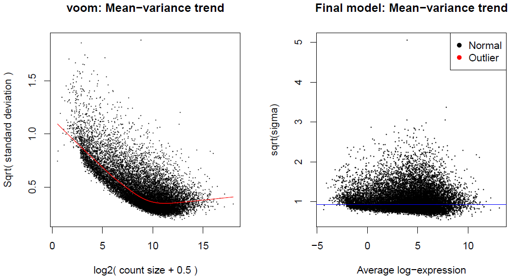
The limma package was initially designed for analyzing intensity data from microarrays. Intensity datasets are essentially continuous numerical experiments, while RNA-seq datasets are a collection of integer counts. The voom()[https://www.rdocumentation.org/packages/limma/versions/3.28.14/topics/voom] method, see the paper⁴ and Chapter 15 in the documentation, provides the necessary statistical properties for the RNA-seq data to be analyzed using the methodological tools developed for microarrays. RNA-Seq data could be analyzed using statistical theory developed for count data, but the underlying mathematical theory of count distribution is less tractable than that of the normal distribution, and there is a problem related to the error rate control with small sample sizes. That being said, applying normal-based statistical tools to RNA-seq count data is not simple, because the counts have markedly unequal variabilities, even after log-transformation. The voom() method finds it crucial to understand the way in which the variability of RNA-seq read counts depends on the size of the counts and addresses the issue by modeling the mean-variance relationship (see Figure 4). In the voom method paper (Law et al., 2014)⁴, two ways of incorporating the mean-variance relationship into the differential expression analysis are explored. The first option, limma-trend analysis, is executed by setting the parameter ‘Trend’ to TRUE in the empirical Bayes function (eBayes) and the second one, limma-voom by using a precision weight matrix combined with the normalized log-counts. limma-trend applies the mean-variance relationship at the gene level whereas limma-voom applies it at the level of individual observations. Both limma-trend and limma-voom perform almost equally well when the sequencing depths are similar for each RNA sample. When the sequencing depths are too different however, limma-voom is the best performer and the one to be used. It is suggested in the limma documentation to use the limma-trend approach when the ratio of the largest library size to the smallest is not more than about 3-fold. In the case of this analysis, the ratio is 3.2 and using limma-voom is therefore the better option.

RNA-seq experiments are often conducted with samples of variable quality. Instead of removing them from the analysis, the alternate apparoach of using voomWithQualityWeights() allows them to still be included by computing and assigning each sample an additional weight measure. See the voomWithQualityWeights() paper⁵ and section 15.6 in the documentation. More precisely, the voomWithQualityWeights approach analyses RNA-seq experiments by assigning a quality weight to each sample. The sample weights are function of the estimated sample variance derived from a log-linear variance model that includes common sample-specific or group-specific parameters. This approach leads to a more powerful analysis and fewer false discoveries compared to conventional approaches. Below you can find the code required to perform the analysis with both voom() and voomWithQualityWeights().
N.B. In the code bellow, voomWithQualityWeights() lines are commented out. They can only be used if voom is not used, in that case it’s important to comment out the voom() lines instead. An additional source of interesting information on when to use one or the other can be found on these question asked on the bioconductor and biostars forums. In this code we also make use of the duplicateCorrelation() function from the limma package. This one is used after one of the voom functions to account for the correlation present between samples from the same individual. For example in this study, there were three regions of interest studied for each mice, therefore there were three different sample collected from the same mouse. It is important do downweigh the effect of higher correlation associated with these three samples. For more information you can refer to this question on the Bioconductor forum.

Voom and Linear Modeling
## Use voom() to convert the read counts to log2-cpm, with associated weights, ready for linear modelling:
v <- voom(dge, design, plot=TRUE)

## If using vWQW:
# v <- voomWithQualityWeights(dge, design, plot=TRUE)

# Estimate the correlation between the brain region cell lines that were extracted from the same mouse subject.
corfit = duplicateCorrelation(v, design, block = dge$samples$subject)

## The intra cell line correlation will change the voom weights slightly, so we run voom a second time:
v <- voom(dge, design, plot=TRUE, block = dge$samples$subject, correlation = corfit$consensus)

## If using vWQW:
# v <- voomWithQualityWeights(dge, design, plot=TRUE, block = dge$samples$subject, correlation = corfit$consensus)

# Similary, we run update the correlation for the new voom weights:
corfit = duplicateCorrelation(v, design, block = dge$samples$subject)

Figure 4: Mean Variance Trend

2.8 Contrasts and Model Fit:

One of the advantages of using limma for RNA-Seq analysis is its ability to accommodate arbitrary experimental complexity. Amongst these features is performing comparisons between groups (log fold-changes), obtained as custom contrasts of the fitted linear models (The UC Davis Bioinformatics RNA-Seq Workshop from June 2018 contains good information and examples of this). Below is a simple control (SAL) vs. condition (POL) contrast.

fit = lmFit(v, design, block = dge$samples$subject, correlation = corfit$consensus)

#### Contrasts
cm = makeContrasts(
  POLvsSAL = POL-SAL,
  levels = design
)

fit2 = contrasts.fit(fit, cm)

2.9 eBayes()

The empirical Bayes method ebayes() assumes a scaled chi-square prior distribution and uses that information to derive posterior values for the variance in the residuals. The moderated t-statistic is computed using that posterior values. The extra information is borrowed from the ensemble of genes for inference about each individual gene. Moderated t-statistics lead to p-values in the same way that ordinary t-statistics do, with the exception of increased degrees of freedom, reflecting the greater reliability associated with the smoothed standard errors. The eBayes function computes one more useful statistic, which is the moderated F-statistic (F). The F statistic combines the t-statistics for all the contrasts into an overall test of significance for that gene. The F-statistic tests whether any of the contrasts are non-zero for that gene, i.e., whether that gene is differentially expressed on any contrast. The denominator degrees of freedom is the same as that of moderated-t. Its p-value is stored as fit$F.p.value. It is similar to the ordinary F-statistic from analysis of variance except that the denominator mean squares are moderated across genes. We ran eBayes with the robust=TRUE parameter to account for gene-level outliers.
fit3 = eBayes(fit2, robust=TRUE)

2.10 Multiple Testing

Limma provides two functions to perform hypothesis tests and adjust the p-values for multiple testing; topTable() and decideTests(), see the limma user’s guide documentation for more details. The basic statistical method used for significance analysis is the moderated t-statistic, which is computed for each probe and for each contrast. The moderated t-statistic is similar to the ordinary t-statistic except that the standard errors have been moderated across genes using a simple Bayesian model implemented by the eBayes() method.

decideTests()

The function decideTests() offers a number of strategies for doing multiple testing across contrasts through its method= parameter. The latter offers four different options: separate, global, hierarchical and nested. The simplest one being the separate method, which is the default option in the decideTests() function. It performs multiple testing for each contrasts separately and is the equivalent of using topTable(). The global method is recommended when a set of closely related contrasts are being tested. This method simply appends all the tests together into one long vector of tests, i.e., it treats all the tests as being equivalent regardless of which probe or contrast they relate to. An advantage is that the raw p-value cutoff is consistent across all contrasts. For this reason, method=”global” is recommended if you want to compare the number of DE genes found for different contrasts, for example interpreting the number of DE genes as representing the strength of the contrast. However users need to be aware that the number of DE genes for any particular contrasts will depend on which other contrasts are tested at the same time. Hence one should include only those contrasts which are closely related to the question at hand. Unnecessary contrasts should be excluded as these would affect the results for the contrasts of interest. Another more theoretical issue is that there is no theorem which proves that the adjust.method=”BH” option, when in combination with the method=”global” parameter, will correctly control the false discovery rates for combinations of negatively correlated contrasts. Nevertheless, simulations, experience and some theory suggest that the method is safe in practice. The hierarchical method offers power advantages when used with adjust.method=”holm” to control the family-wise error rate. However its properties are not yet well understood with adjust=”BH”. The method=”nestedF” method has a more specialized aim in giving greater weight to probes which are significant for two or more contrasts. Most multiple testing methods tend to underestimate the number of such probes. There is some practical experience to suggest that the method=”nestedF” method is less conservative when finding probes which respond to several different contrasts at once. However this method should still be viewed as experimental. It provides formal false discovery rate control at the probe level only, not at the contrast level. The decideTest() results can be output in a clear manner using the R ktable() function.

topTable()

topTable() summarizes the results of the linear model and a gives a number of summary statistics for the top genes and selected contrast. The output from topTable includes an adjusted p-values column which displays the multiple testing result. By default, topTable and other Limma functions use Benjamini and Hochberg’s method (BH) to control the false discovery rate. Notice that the topTable() function handles the contrasts separately. That being said, using it to test a set of contrast together will give the same results as when each contrast is tested on its own. topTable does not perform any multiple testing adjustments between contrasts, hence the raw p-value cutoff can be very different for different contrasts, depending on the number of DE probes. This method is recommended when different contrasts are being analysed to answer more or less independent questions.

dt <- decideTests(fit3, method="separate")
# To make the output nice:
kable(t(summary(dt)))

top.table <- topTable(fit3, sort.by="P", n=Inf, adjust.method="BH")

kable output:

|         | Down| NotSig|  Up|
|:--------|----:|------:|---:|
|POLvsSAL |  560|  14225| 240|

N.B.: The topTable() parameter sort.by= is set to “P”, as explained in the function’s documentation, this sorts the results by p-values and therefore returns a ranked list (see the Pathway Enrichment Analysis page for more details on this).

2.11 Saving to file:

If single comparison (from above):
write.csv(top.table, file="../DE_results_folder/POLvsSAL.csv", row.names=F)

To save a partial ranked list (see above and the Pathway Enrichment Analysis page) one can filter the top.table results. Here’s an example of two partial output from the results, up-regulated gene and down-regulated genes only, filtered by value being above or below 0.1 logFC and with an adjusted p-value bellow 0.05:

write.csv(top.table[which(top.table$adj.P.Val < 0.05 & top.table$logFC > 0),], file="../../data_files/limma_voom/POLvsSAL_UP_DEGs.csv")

write.csv(top.table[which(top.table$adj.P.Val < 0.05 & top.table$logFC < 0),], file="../../data_files/limma_voom/POLvsSAL_DOWN_DEGs.csv")

In case of multiple comparisons made (See 2.7 Contrasts and Model Fit):

for (c in colnames(dt)) {
  
  degs = topTable(fit2, coef = c, n=Inf, sort.by = 'P', adjust.method='BH')
  
  write.csv(degs, file=paste0("../DE_results_folder/", c, ".csv"), row.names=F)
}

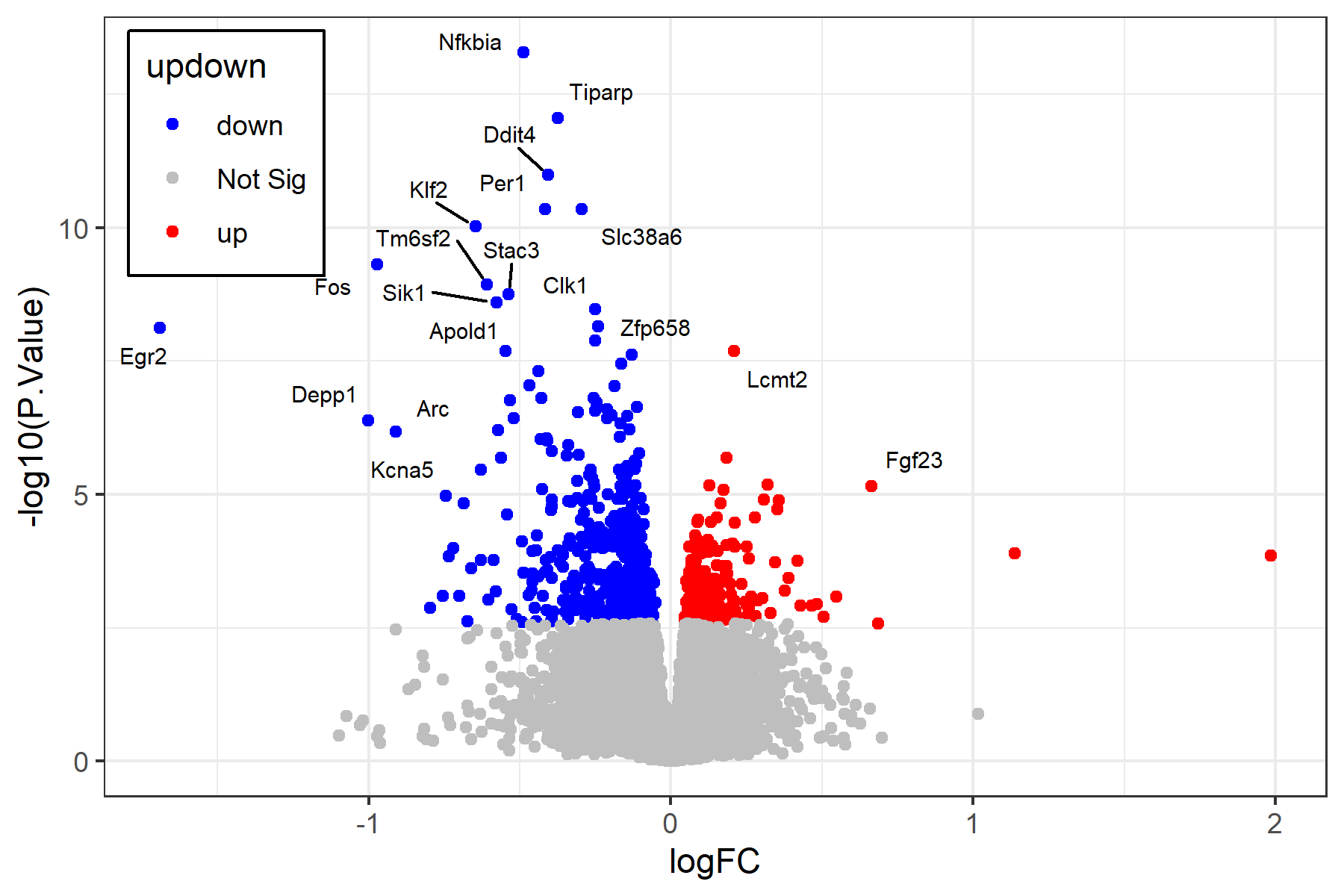
See POLvsSAL.csv for a sample output top.table file.

Also see the volcano_plot.r file for a script that can generate a volcano plot similar to the one below for this analysis. See the sample_figures page for example outputs.

Figure 5: Example Labeled Volcano Plot

---

1. Law, C. W., Alhamdoosh, M., Su, S., Dong, X., Tian, L., Smyth, G. K., & Ritchie, M. E. (2016). RNA-seq analysis is easy as 1-2-3 with limma, Glimma and edgeR. F1000Research, 5. ↩ ↩² ↩³

2. Chen, Y., McCarthy, D., Ritchie, M., Robinson, M., Smyth, G., & Hall, E. (2020). edgeR: differential analysis of sequence read count data User’s Guide. Accessed: Jul, 8. ↩

3. Robinson, M. D., & Oshlack, A. (2010). A scaling normalization method for differential expression analysis of RNA-seq data. Genome biology, 11(3), 1-9. ↩ ↩²

4. Law, C. W., Chen, Y., Shi, W., & Smyth, G. K. (2014). voom: Precision weights unlock linear model analysis tools for RNA-seq read counts. Genome biology, 15(2), 1-17. ↩ ↩²

5. Liu, R., Holik, A. Z., Su, S., Jansz, N., Chen, K., Leong, H. S., … & Ritchie, M. E. (2015). Why weight? Modelling sample and observational level variability improves power in RNA-seq analyses. Nucleic acids research, 43(15), e97-e97. ↩