Pre-Processing Steps
Pre-Processing Steps
The pre-processing steps starts with raw sequencing data (usually in fastq.gz format)
1. Pre-Alignment Quality Control (QC)
Multiple programs can be used to perform quality control. Here we will use FastQC and MultiQC.
1.1 FastQC
Run the program on the raw read files to return a QC report.
Depending on your system, you can use a bash command similar to the following:
fastqc -t 12 raw_data/* -o fastqc_output/
Here the raw data is located in the raw_data/ folder and the output (one for each data file will be in the fastqc_output/ folder). You can find a example of a FastQC output here.
Sometimes there are information contained in the read file name, in this case it contains the company NEB (New England Biolabs) and the fact that the read are paired-end. R1 means this is the first of the two pairs. See the Study Design page.
1.2 MultiQC
Run the program from anywhere within your project folder. MultiQC will automatically recognize file extensions and organize its report with the right files in each section.
Depending on your system, you can use a bash command similar to the following:
multiqc . -o multiqc_output/
The output will consist of only one html file and will be located in the multiqc_output/ folder). You can find a example of a MultiQC output here.
Sometimes there are information contained in the read file name, in this case it contains the company NEB (New England Biolabs) and the fact that the read are paired-end. R1 means this is the first of the two pairs. See the Study Design page.
1.3 Assessing the results
Before continuing with the pipeline it is important to use these first QC results to understand how good the metrics are in our experiment and if any further investigations into the data or the experimental protocol is required. FastQC contains multiple sections in it’s results which it will flag in red or yellow if it detects something seems off the norm. This can actually be expected depending on what experiment is being run. FastQC’s checks are built for a very standard experiment, but all experiment are unique. MultiQC is very good at providing a bird’s eye view of the fastQC results for all samples. This is very helpful to check wether the same issues of flags are raised in the other samples or only a single one or a few.
Two excellent resources to consult when assessing FastQC results is the fastQC documentation and the QCFail blog, run by the folks at the The Babraham Institute in Cambridge, the team that actually developed FastQC. Of course, a google search and most notably the SEQanswers and the Biostars online communities are also a great help.
FastQC divides its report into modules, of which it will assign a color according to the following logic: normal (green tick), slightly abnormal (orange triangle) or very unusual (red cross).
Let’s go through the flags return in our example real-life FastQC results.
The following three sections were flagged, 2 of them as abnormal and one as slightly abnormal:
1.3.1 Per Base Sequence Content
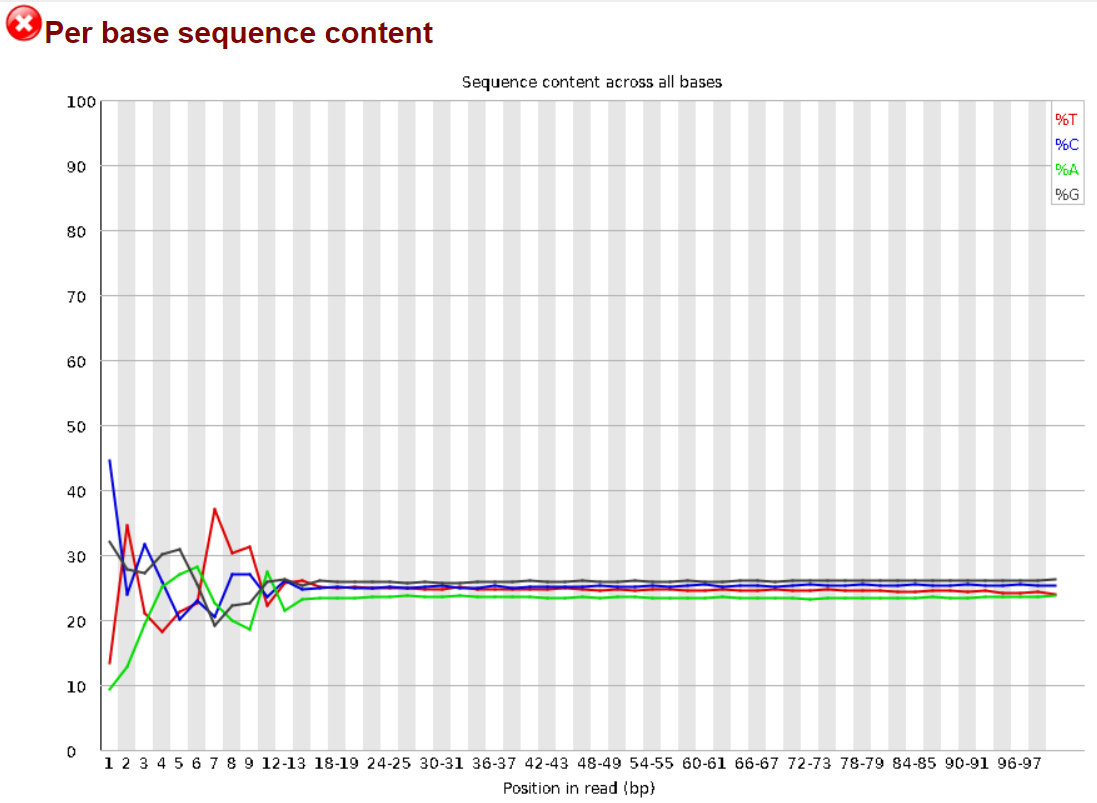
In theory, all reads from a sequencing sample should contain approximately the same ratio of the 4 bases across their sequence. FastQC is designed to flag samples in which this is not the case. Here we see that the first 10-12 bases in the reads from this sample fail to respect this assumption. A search on the web quickly points to this Biostars discussion linking to this QCFail blog post by Dr. Simon Andrews, which reassure and explains the existence of this bias as being caused by the random priming step in library production. (See random primers in the Glossary). In his own words:
The priming should be driven by a selection of random hexamers which in theory should all be present with equal frequency in the priming mix and should all prime with equal efficiency. In the real world it turns out that this isn’t the case and that certain hexamers are favoured during the priming step, resulting in the based composition over the region of the library primed by the random primers.
Also:
Ironically if you are producing RNA-Seq libraries it would make for better QC if you were to focus on libraries which didn’t have this artefact in them, as they would be the ones which were truly suspicious.
We a bit more research on can find tools capable of removing this bias in case this is needed, for example Genominator:
1.3.2 Per Sequence GC Content.
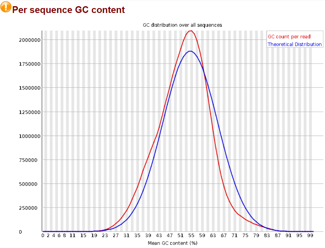
GC content should follow a normal distribution across the reads in the sample. Here FastQC is only flagging it as slightly abnormal, we will still look into it. The first check is to make sure it follows a normal curve, which here it almost does, some analyses will return graphs with very odd distributions as Dr. Simon Andrew addresses in this other blog post on the QCFail blog. Here the somewhat higher GC content in the sample can be explained by it being mice data. The mouse genome contains a GC concentration slightly higher than other species (e.g.: 51% for mice vs. 46% for humans).1
1.3.3 Sequence Duplication Levels
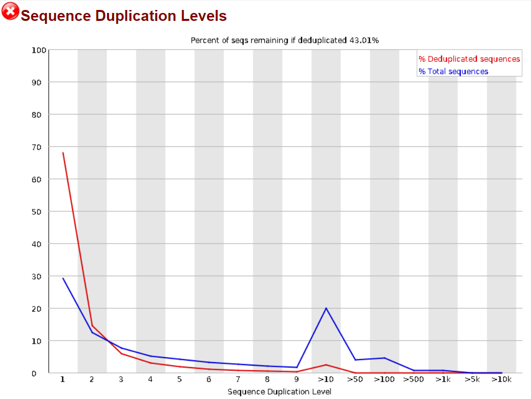
FastQC performs a read duplication check to make sure that the sample is not contaminated by external sequences or PCR enrichment bias. See the FastQC documentation on duplicate sequences, this very excellent Biostars answer by Dr. István Albert and Dr. Simon Andrews personal blog’s (Proteo.me.uk) post on the same topic for more information on why this can be expected and what are its possible causes.
This is also explained by FastQC starting to show it’s age and being outdated for paired-end sequencing as this article from the UC Davis Genome Center’s DNA TECH (DNA Technologies & Expression Analysis Core) website addresses, recommending instead the use of more modern tools such as HTStream and FASTP for paired-end data.
2. Adapter Trimming:
Adapters are usually provided in the experiment meta data since the information is part of library preparation. Adapters are present on the reads as part of the sequencing protocol, they usually contain the sequencing primer binding sites, the index sequences, and the sites that allow library fragments to attach to the flow cells. They are usually found on the 3’ end of sequences, this might vary. Just as PCR primers (see glossary) they are artificial DNA oligonucleotides and will oftentimes, depending on the experimental protocol, remain on raw read sequences and must therefore be removed for obvious reasons. Multiple tools have been developed for this, here we show how to use Cutadapt.2
Here’s an example with made-up adapters:
adapter1 = ATGAGTGACACGTCTGAACTCCAG
adapter2 = AGAGCCACGTCTGAACTCCAGAGG
cutadapt --cores=12 -q 30 -m 20 -a ATGAGTGACACGTCTGAACTCCAG -A AGAGCCACGTCTGAACTCCAGAGG ../raw_data/R1.fastq.gz ../raw_data/R2.fastq.gz > cutadapt_output/cutadapt_report.txt
Parameters:
- –cores parallelizes the task over a specific number of cores
- -q instructs the program to discard reads with a Phred score < 30 (see the glossary for more information on Phred scores)
- -m tells it to discard reads < 20bp
- -a is for a Regular 3’ adapter (R1)
- -A its paired read (R2)
- -o the output R1 file
- -p the output R2 file
- This is then followed by the respective input files and the Standard output (stdout) to a report file. N.B.: Of course you can run this with the scripting program of your choice and modify the file suffixes to match the each sample.
3. Alignment
The alignment phase consists in the mapping of the sequenced reads to an organism’s genome to determine where in the genome they originated from. This can be achieved with multiple tools. In this tutorial we’re using STAR (Spliced Transcripts Alignment to a Reference).3 As the name entails is an aligner that’s able to account for splicing. It is also faster than most of its counterparts and can run on somewhat less resources. The use of a server instead of you own PC would still be recommended however, depending on the library and the genome sizes. For more information the Bioinformatics Training at the Harvard Chan Bioinformatics Core provides a great explanation of how the STAR algorithm works.
3.1 Index Generation
The first step in using STAR is generating and index for the genome used in the study. This allows alignment to be performed faster. Here’s a sample command for generating an index for the Mouse genome. In this study we’re using the mm10 GRCm38.p6 GCA_000001635.8 mouse genome assembly. You can also download the genome files (.FA, .GTF, etc.) from the ensembl website.
Here’s an example command for index generation:
STAR --runMode genomeGenerate --runThreadN 8 --genomeDir star_index --genomeFastaFiles Mus_musculus.GRCm38.dna_sm.toplevel.fa --sjdbGTFfile Mus_musculus.GRCm38.102.gtf --sjdbOverhang 99
To better understand the STAR command parameters you can refer to the latest STAR Manual and to this thread on Biostars.
3.2 Alignment with STAR
Here’s an example command for performing alignment with STAR:
STAR --genomeDir mm10/star_index --readFilesIn raw_data/R1_trimmed.fastq.gz raw_data/R2_trimmed.fastq.gz --readFilesCommand zcat --runThreadN 12 --outFilterIntronMotifs RemoveNoncanonicalUnannotated --outSAMtype BAM SortedByCoordinate --outSAMstrandField intronMotif --quantMode GeneCounts --outFileNamePrefix STAR_results/
As with the Index creation, to choose and understand the parameters refer to the latest STAR Manual. No experiment is designed equal therefore different parameters cna be used for every situation. When in doubt simple use the defaults, they’re already well thought of.
4. Post-Alignment Quality Control
Quality control of the mapped reads can be performed using MultiQC by running again the same command as for the pre-alignment QC:
multiqc . -o multiqc_output/
MultiQC will automatically add a module with information about the mapped reads in its report.
Interesting checks to make about the data are:
- Is the alignment rate at least 80%
- Is there an even gene body coverage
- Are there too many intronic/intergenic reads
These three points are taken from this excellent answer by Dr. Friederike Dündar on Biostars. There are many reasons why some of them might fail, from experimental errors in library preparation and/or the alignment pipeline or sample contamination from other species or ribosomal RNA (rRNA).
Example of other tools that can be used to further investigate and also perform post alignment QC are RSeQC, QoRTs and the Broad Institute’s Picard.
-
Romiguier, J., Ranwez, V., Douzery, E. J., & Galtier, N. (2010). Contrasting GC-content dynamics across 33 mammalian genomes: relationship with life-history traits and chromosome sizes. Genome research, 20(8), 1001-1009. ↩
-
Martin, M. (2011). Cutadapt removes adapter sequences from high-throughput sequencing reads. EMBnet. journal, 17(1), 10-12. ↩
-
Dobin, A., Davis, C. A., Schlesinger, F., Drenkow, J., Zaleski, C., Jha, S., … & Gingeras, T. R. (2013). STAR: ultrafast universal RNA-seq aligner. Bioinformatics, 29(1), 15-21. ↩